Molecule Builder
The Molecule Builder section of MAD is the main entry point to obtain the coarse grained
representation of your molecule of interest.
Its most basic feature, is a wrapper around the
vermouth-martinize[1] software.
In practice, the MAD:Molecule Builder introduces many powerful features,
such as interactive edition of distance constraints,
that facilitate and add controls to the coarse graining process.
The following topics will be covered in order to guide you through your first use of the MAD:Molecule Builder.
1. Classic mode with a single chain molecule
2. Protein with elastic network
3. Protein with GO model
4. Browse my builds through history
person_add
Because the MAD:Molecule Builder makes use of
our computational resources, it is required
that you sign in in order to have access it.
Classic mode with a single chain protein
Upon authentication to the MAD website,
the Molecule Builder option
should toggle to black, marking it as accessible.
Click on it to access to the MAD:Molecule Builder welcome page.
Here you will be invited to upload a coordinate file.
launch
The MAD:Molecule Builder requires a single PDB file as input.
We will use as example, the Neisserial surface protein A (NspA) from the bacterium Neisseria
meningitidis, which forms a transmembrane beta barrel.
It is a single chain membrane protein.
Its atomistic structure can be downloaded from the PDB web
site under the code 1P4T.
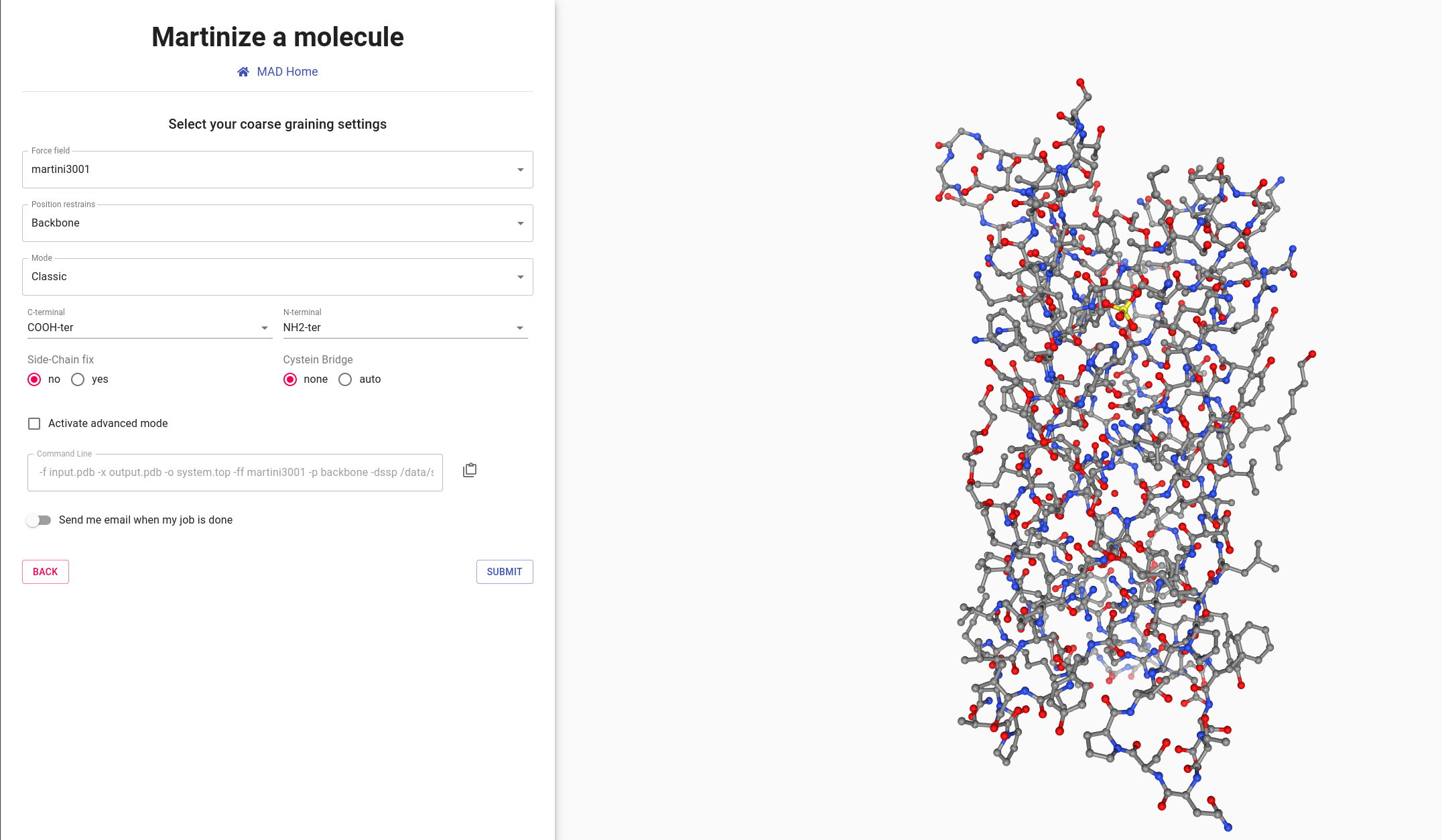
Once loaded, the all atom structure is displayed and the interface displays
several options to configure the coarse-graining process of the structure.
- Force field: choose the version of MARTINI that you plan to use during your molecular dynamics simulation.
- Position restraints: generally useful during the equilibration simulation of the molecule, in order to maintain the structure of the backbone.
- Mode: Search for molecule within the selected biochemical category
- termini and fixes: patches molecular beads to improve representations of functional groups charges and geometries.
- Cystein bridges: detect and apply covalent bonds between cysteine side-chains based on distances.
- Email: In case of a long running computation, email can be sent upon completion. The email will enclose a link to access and visualize your data. Your data are privately stored on the server for a period of 15 days.
launch
Set the force field parameter to the 3.0.0.1 version of Martini.
We will use the classic mode, alternative modes will be explored later on.
All remaining options will be left in default state: neutral termini, no side-chain fix, and no cysteine
bridge.
Then proceed to the submission of the protein.
The MAD:Molecule Builder should take a few seconds to generate a MARTINI model of
NspA.
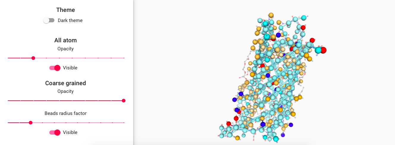
Feel free to explore the several representation options provided to visualize the newly coarse-grained protein.
- Change the beads radius by a factor
- Select other representations such as surface.
- Modify all atoms and coarse grain representation opacities.
- Set Bead radius scaled according to Martini 3 definitions.
info_outline
Martini 3 force field has 3 bead sizes which are mainly defined by the number
of non-hydrogen atoms represented by the bead:
regular (R) size for 4 atoms mapped by 1 bead (or 4-1),
small (S) size for 3-1 and tiny size(T) for 2-1 mappings.
The unscaled radius of the R, S and T beads in Martini 3 corresponds to 0.264, 0.230 and 0.191 nm, respectively.
Color scale goes from cyan to white to orange to show hydrophobicity of beads.
Cyan beads have low hydrophobicity value and orange beads have high hydrophobicity value.
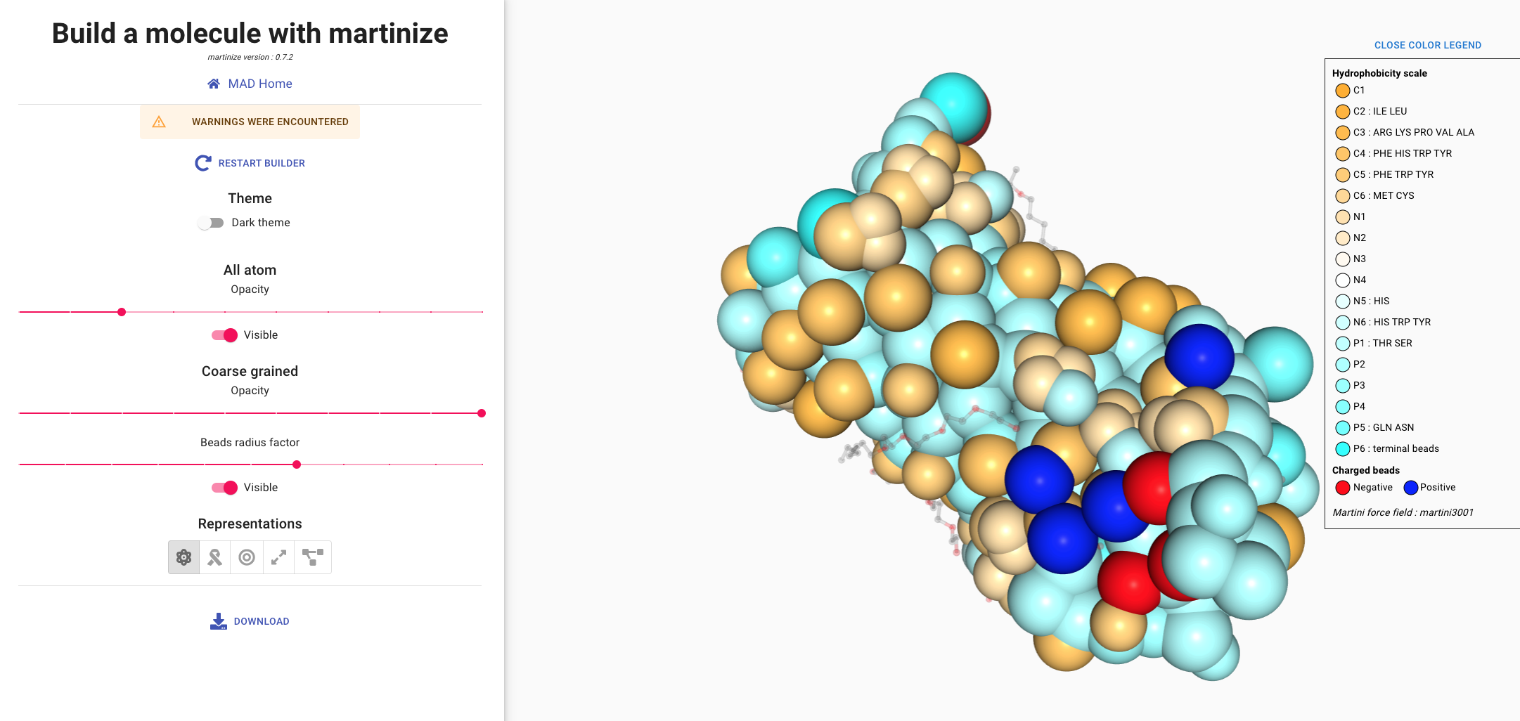
info_outline
The Martini3 model features 3 main chemical classes of neutral beads: C for apolar/ hydrophobic,
N for intermediate and P for polar/hydrophilic.
Each class has 6 beads with a number as suffix. This number represents the degree of hydrophobicity of
the bead: ranging from 1 (more hydrophobic) to 6 (less hydrophobic).
The color scale represents the hydrophobicity. As a rule of thumb, C beads will be represented by
orange hues, N by white and P by cyan.
info_outline
There are 2 classes of charged beads in MARTINI 3: Q beads for monovalent +1/-1 charged
molecules and D beads for divalent charged molecules.
While Q beads also have five degrees of hydrophobicity,
the color code for charged beads in MAD will only account for the sign of the charge.
Positively charged beads are blue and negatively charged beads are red.
Protein with elastic network
The elastic network approach consist of a set of harmonic potentials added on top of
the Martini model to conserve the tertiary structure of proteins.
The network is fully dependent of the pdb structure used as reference, with
the number of bonds defined by the upper and lower distance cutoff.
The rigidity of the protein model is defined by the number of elastic bonds and by the force constant used.
Optimal parameters for the elastic network depend of the protein system in study.
It is recommended to use experimental or atomistic simulations data to calibrate the parameters of your
elastic network.
To illustrate the interests of the elastic network tool in MAD:Molecule Builder
we will use the T4 Lysozyme protein from the bacteriophage T4.
launch
Download the corresponding PDB structure.
Then, go back to the MAD:Molecule Builder welcome screen and load this file.
For T4 Lysozyme in MARTINI 3, after setting Force field to "martini3001" and Mode to "Elastic", we recommend the following parameters:
- A force constant of 700 kJ/(mol.nm2)
- Lower and upper cutoff of 0.5 and 0.9 nm respectively
- Use neutral termini, side-chain fix, and auto assignment of cysteine bridges
- Activate the side chain fix
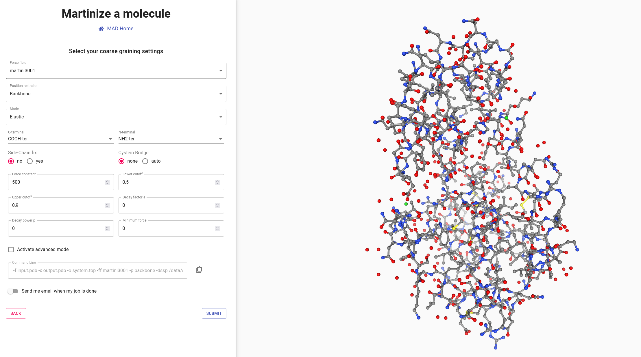
info_outline
Additional improvements of the protein stability and reliability of its structures and dynamics are achieved
by applying the side chain fix option, which adds dihedral angles between SC1-BB-BB-SC1 beads, leading to an
improvement of the overall side chain orientations.
launch
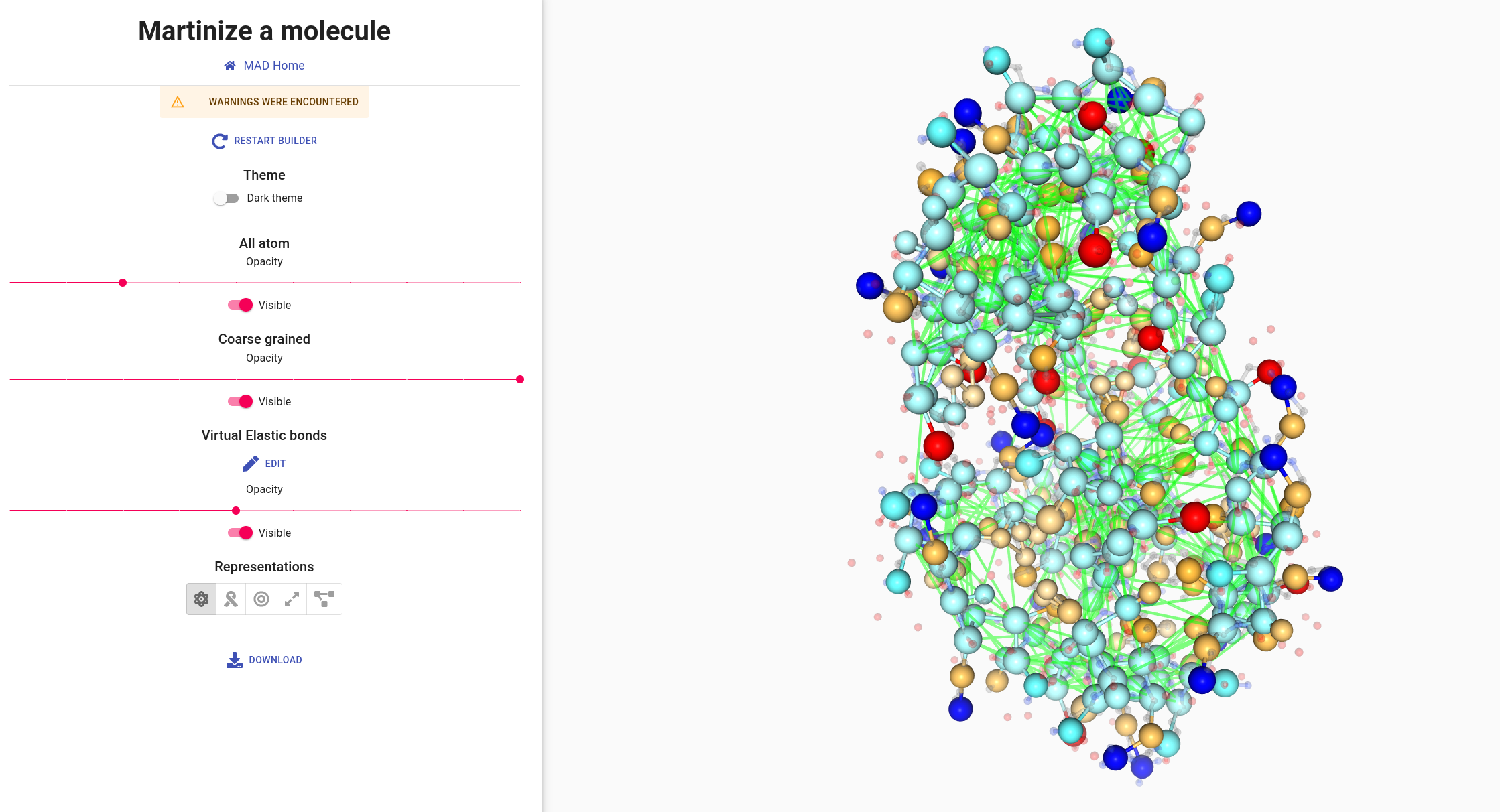
The protein is ready to be coarse grained. Click on the SUBMIT and wait for the processing to finish.
You should have access to a viewer of the coarse grained protein with its elastic network represented by green links between beads.
The MAD:Molecule Builder provides two edition modes of the elastic network.
- Manual edition: click on a single bead to remove all its elastic bonds, or add a new bond by clicking on another bead. A direct click on a bond allows to delete it.
- Group selection: select a group of beads and linking them all together, or select two groups to add elastic bonds between each other beads.
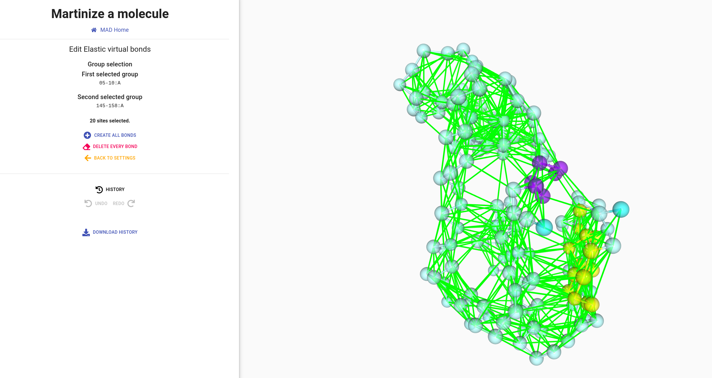
info_outline
The group selection tool implements a simple query language. For example, selecting “05-10:A” as group 1 and
“145-158:A” as group 2, will toggle links between the two groups.
launch
Click on the EDIT button to experiment with the edition modes as
depicted in the pictures around
Single atom click
Direct bond click
Group links edition


info_outline
Once your modifications are done, the MAD:Molecule Builder will ask for a
confirmation before writing them to your history. Should you accept, the previous elastic model will be
erased.
Nothing prevents you from relaunching a Molecule Builder with the same file if you want to have different
network states for the same molecule.
Protein with GO model
The same way as for Elastic network, you can generate martinize protein with Go bonds.
The Go model approach implemented in Martini protein models have two main differences
in relation to elastic network approaches: the type of potential function used and
how the contact map is defined.
For the potential function, instead of the harmonic potentials used in elastic approaches,
the approach is based on a dissociative Lennard-Jones potential, which is placed on virtual
sites built based on the position of the backbone beads (see the GROMAC manual for more
details on virtual sites).
The contact map in Go models are not necessarly only defined by distances cutoff between backbone
beads and more sophisticated criterion can be employed. The implementation of Go models
used with Martini is based on a contact map formed by the combination of the atomic overlap
criterion (OV), a variant of the contact of structure units (CSU)[1] and
a geometrical occlusion method.
Independent of the contact map approach used, calibration of dissociation energies and cutoff
based on experimental and/or atomistic simulation data are recommended.
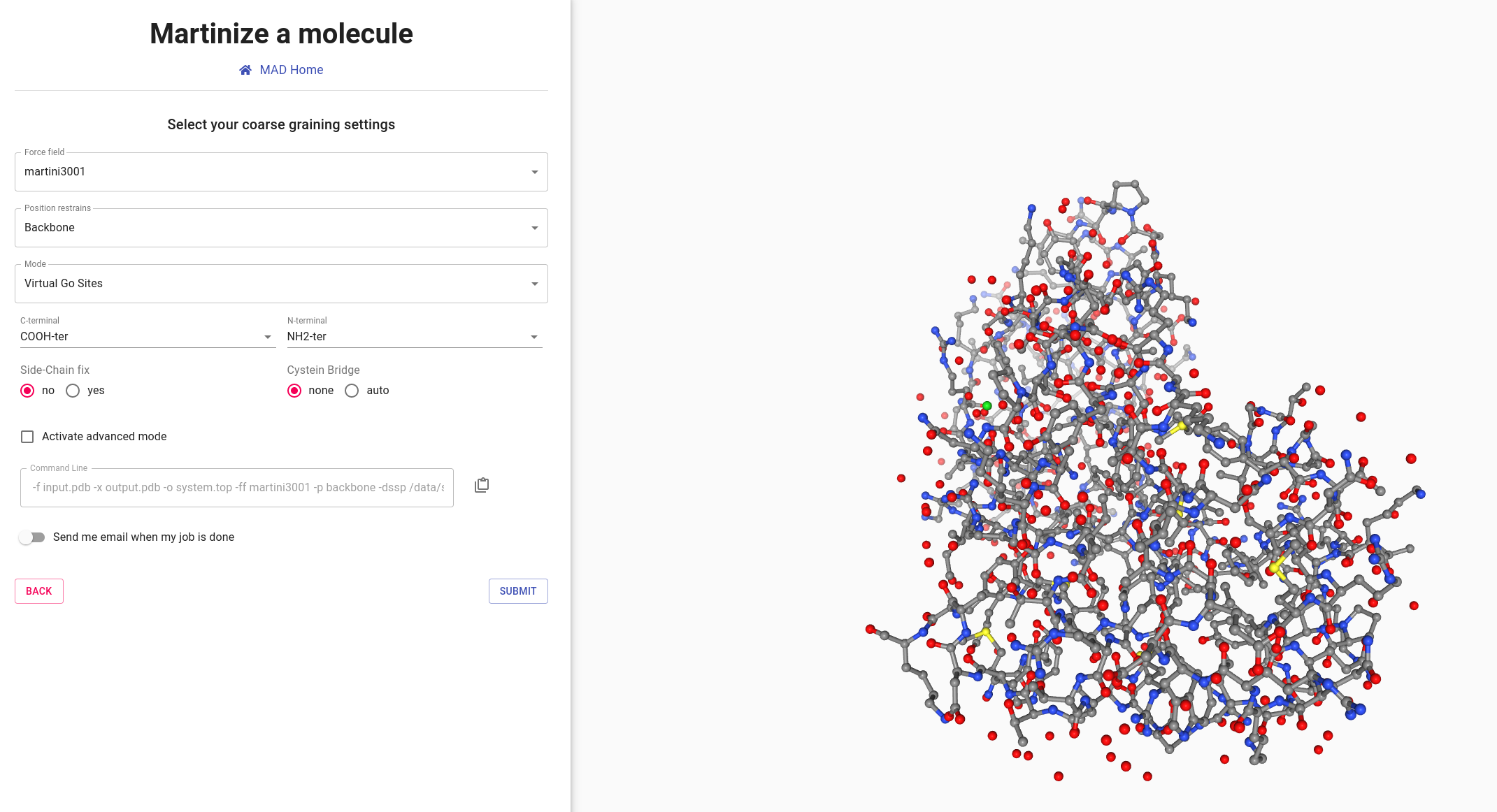
launch
Go back to the MAD:Molecule Builder welcome screen and load T4 Lysozyme protein file again.
Select Virtual Go sites option, other options remaining as default.
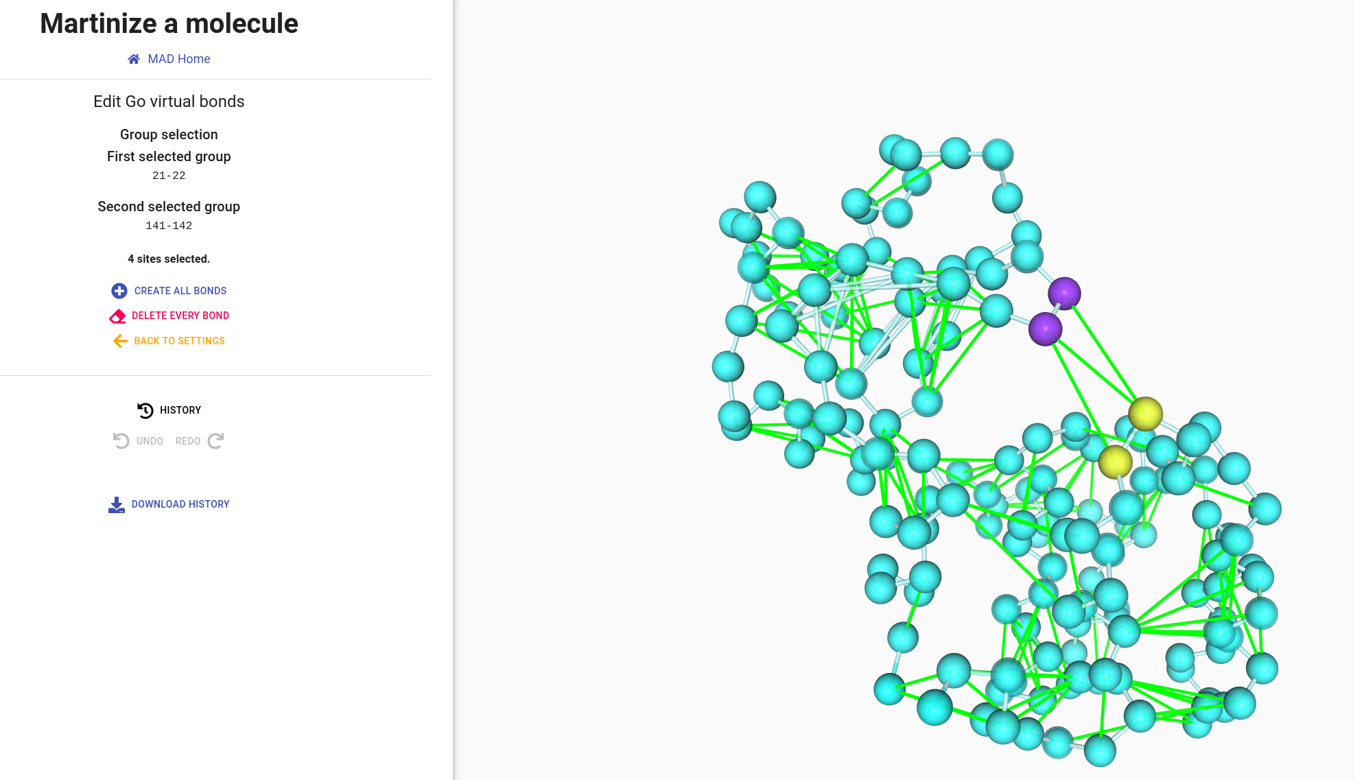
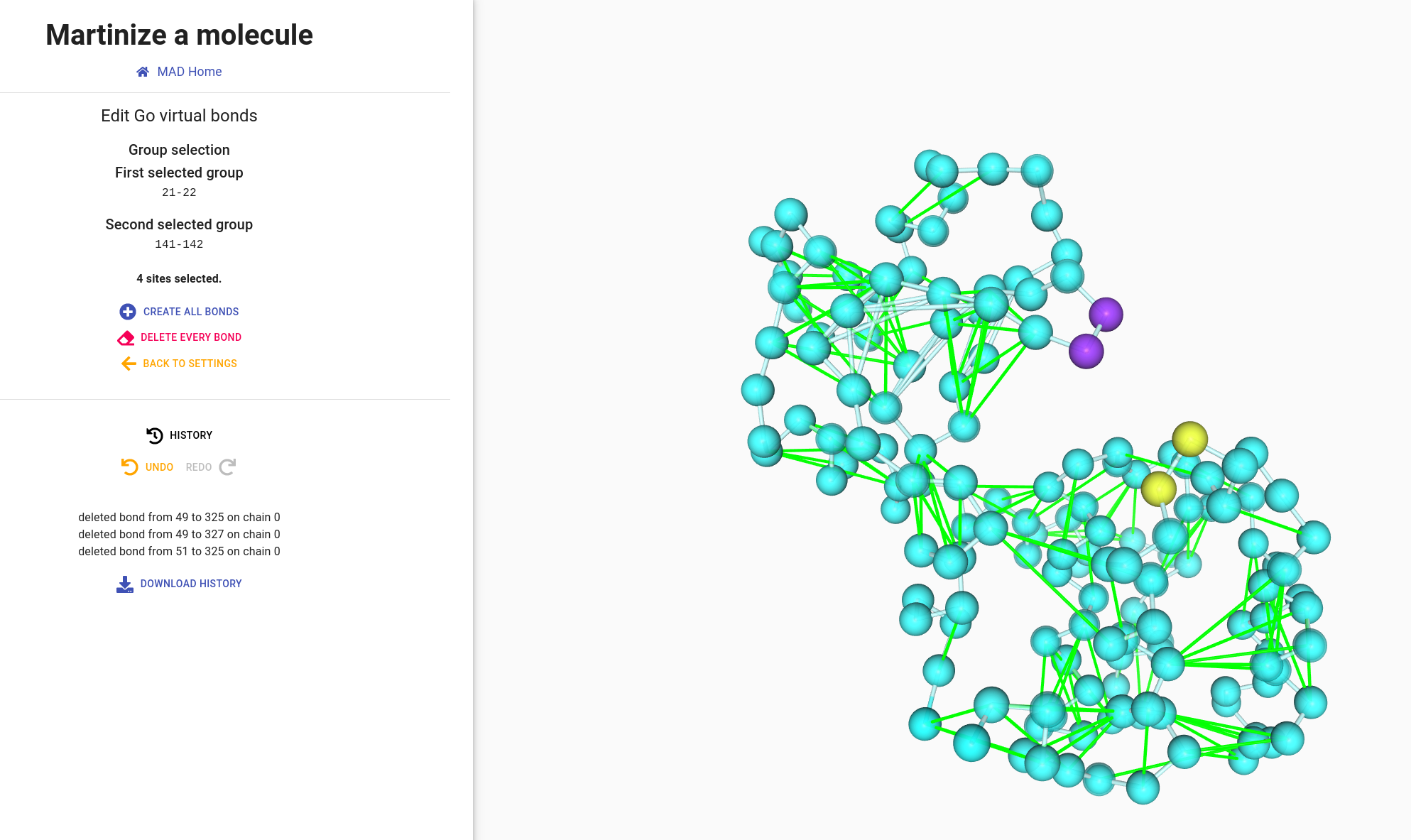
The representation of GO bonds is similar to elastic bonds. You can interact with bonds the same way by clicking to select one bond, one bead or an entiere group.
launch
We can select group 21-22 and group 141-142 to remove all bonds between them.
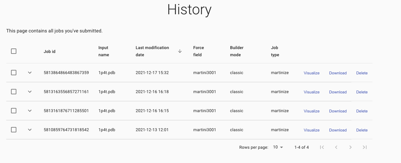
Browsing my molecular builds through history
Click on My builder history in the left-end menu,
to access to all your previous builds made with the MAD:Molecule Builder.
Access an individual model to reload it for further editing or to download the result files.
A detailed description of each build can be displayed by clicking on the down arrow.
info_outline
As any element of your history, the molecule will also be available
into MAD:System Builder for its integration into larger system.
References
- Poma, A. B., Cieplak, M. & Theodorakis, P. E. Combining the MARTINI and structure-based coarse-grained approaches for the molecular dynamics studies of conformational transitions in proteins. J. Chem. Theory Comput. 13, 1366–1374 (2017)